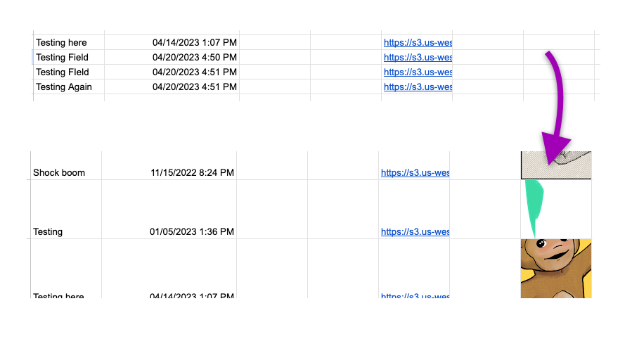
Hey there, spreadsheet enthusiasts! Ready to take your Google Sheets game to the next level? Today, we're diving into the awesome world of the =IMAGE function! If you're tired of plain old numbers and text in your spreadsheets and want to spice things up with some visuals, this function is your ticket to spreadsheet stardom.
First things first, the =IMAGE function does exactly what it says on the tin: it lets you insert images directly into your spreadsheet cells. No more boring columns and rows – let your creativity shine by adding pictures that bring your data to life!
Here's the lowdown on how to use it:
Step 1: Set Up Your Spreadsheet
Open up Google Sheets and fire up a new or existing spreadsheet where you want to add images. Got it? Great! Now, pick a cell where you want the image to appear. This could be in any cell of your choosing.
Step 2: Type in the =IMAGE Function
In the cell you selected, type in =IMAGE("URL"), replacing "URL" with the actual web address of the image you want to insert. It could be an image from the web or one you've uploaded to a cloud storage service like Google Drive. Remember to enclose the URL in quotation marks!
For example:
=IMAGE("https://link-to-your-image.com/your-image.jpg")
Step 3: Voila! Your Image Appears
Hit Enter after typing the function, and boom! Your chosen image magically appears in the cell you selected. It's like adding a dash of visual awesomeness to your spreadsheet canvas.
Tips and Tricks:
- Resize Images: Don't like the default size of the image? No worries! You can resize it by adjusting the height and width within the function. For instance, =IMAGE("URL", 4, 200, 150) sets the image's height to 200 pixels and width to 150 pixels.
4tells the function that you want to set a specific size for your image. - Cell Adjustments: Need the image to fit perfectly within the cell? Use the cell's width and height adjustments to make sure the image looks just right.
- Dynamic Image Links: If your spreadsheet data includes URLs of images that change, you can link the =IMAGE function directly to the cell containing the image URL. For example: =IMAGE(A2), assuming cell A2 contains the image URL.
Some Caveats:
- Image Hosting: Ensure the image you're linking to is publicly accessible. Images stored on private servers or behind login walls might not display.
- HTTPS and Direct Links: Make sure your image links start with "https://" and are direct links to the image file (e.g., ".jpg", ".png", ".gif").
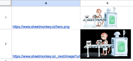
- Transparency: If you want your image to be transparent you must make sure it's a transparent png and you must also make sure that your url ends with
.pngor.gifotherwise Google Sheets will apply a black background to your transparency. Google will also render transparentwebpimages with a black background applied.
 Example of how Google Sheets handles transparent images with urls that don't end in a file extension
So, there you have it – a quick and easy guide to using the =IMAGE function in Google Sheets! Go ahead, add some visual flair to your spreadsheets, and impress your colleagues or friends with your newfound spreadsheet wizardry!
Now, get out there and make those cells pop with pizzazz! 🌟✨
Happy spreadsheet decorating!