Quick Reference: Google Sheets Date Formats
Copy the formula, replace A1 with your cell reference, and you're done.
| Format You Want | TEXT() Formula | Example Output |
|---|---|---|
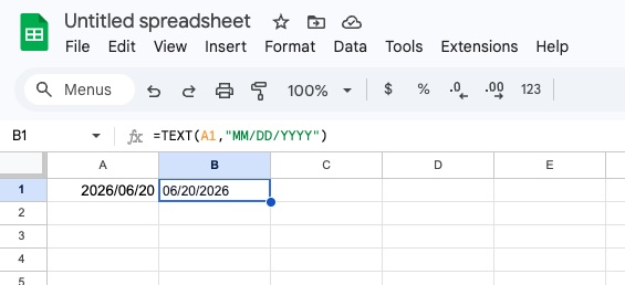
| MM/DD/YYYY | =TEXT(A1,"MM/DD/YYYY") | 04/13/2026 |
| DD/MM/YYYY | =TEXT(A1,"DD/MM/YYYY") | 13/04/2026 |
| YYYY-MM-DD (ISO 8601) | =TEXT(A1,"YYYY-MM-DD") | 2026-04-13 |
| Month D, YYYY | =TEXT(A1,"MMMM D, YYYY") | April 13, 2026 |
| DD-MMM-YYYY | =TEXT(A1,"DD-MMM-YYYY") | 13-Apr-2026 |
| MM/DD/YY | =TEXT(A1,"MM/DD/YY") | 04/13/26 |
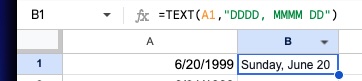
| Day, Month DD | =TEXT(A1,"DDDD, MMMM DD") | Monday, April 13 |
| D-MMM | =TEXT(A1,"D-MMM") | 13-Apr |
| HH:MM AM/PM | =TEXT(A1,"HH:MM AM/PM") | 02:30 PM |
| YYYY-MM-DD HH:MM | =TEXT(A1,"YYYY-MM-DD HH:MM") | 2026-04-13 14:30 |
| Unix timestamp | =INT((A1-DATE(1970,1,1))*86400) | 1776268800 |
For the current date or time, use =TODAY() or =NOW() instead of a cell reference.
How to Format Dates in Google Sheets (3 Methods)
There are three ways to change how dates appear: the Format menu (easiest), the TEXT() function (most flexible), and custom number formats (best for reuse).
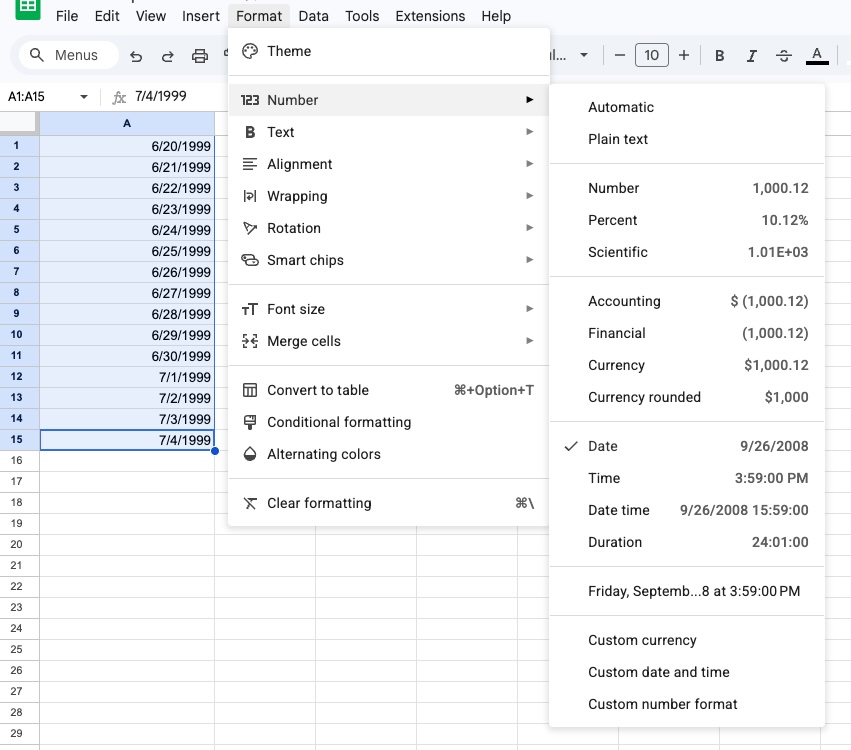
Method 1: Format Menu (Easiest)
This changes how a date is displayed without changing the underlying value. Your formulas and sorting still work normally.
- Select the cells containing dates (or click a column header to select all)
- Go to Format → Number in the top menu
- Choose Date, Time, or Date time
- For more options, click Custom date and time at the bottom of the list
Google Sheets applies the format instantly. You can also right-click the selected cells and choose Format cells to reach the same options.
Method 2: TEXT() Function (Most Flexible)
The TEXT() function converts a date into formatted text. It's the best option when you need to combine a date with other text or export a specific format.
Syntax:
=TEXT(date_value, "format_string")
Examples:
| Formula | Result |
|---|---|
=TEXT(TODAY(),"MM/DD/YYYY") | 04/13/2026 |
=TEXT(TODAY(),"MMMM D, YYYY") | April 13, 2026 |
=TEXT(TODAY(),"DDD") | Mon |
=TEXT(NOW(),"YYYY-MM-DD HH:MM:SS") | 2026-04-13 14:30:45 |
=TEXT(TODAY(),"DDDD") | Monday |
="Report generated: "&TEXT(NOW(),"MMM D, YYYY") | Report generated: Apr 13, 2026 |
Important: TEXT() returns a string, not a date. You can't sort or calculate with the result. Use it for display only — keep the original date in another cell if you need to reference it.
All format codes:
| Code | Meaning | Example |
|---|---|---|
D | Day without leading zero | 3 |
DD | Day with leading zero | 03 |
DDD | Day of week abbreviation | Mon |
DDDD | Full day of week | Monday |
M | Month without leading zero | 4 |
MM | Month with leading zero | 04 |
MMM | Month abbreviation | Apr |
MMMM | Full month name | April |
YY | 2-digit year | 26 |
YYYY | 4-digit year | 2026 |
HH | Hour (24-hour) | 14 |
hh | Hour (12-hour) | 02 |
MM | Minutes (after hour) | 30 |
SS | Seconds | 45 |
AM/PM | AM or PM indicator | PM |
Heads up: MM means months when it appears before a day code, and minutes when it appears after an hour code. Google Sheets figures out which one you mean based on context.
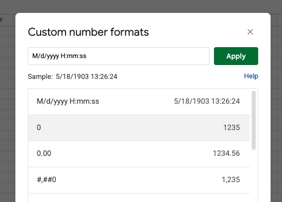
Method 3: Custom Number Format (Best for Reuse)
Custom number formats change how the cell is displayed without converting to text. The date value stays intact for sorting and formulas.
- Select the cells containing dates
- Go to Format → Number → Custom number format
- Type your format string (e.g.,
YYYY-MM-DDorDD/MM/YYYY HH:MM) - Click Apply
This format persists — any new date you type in the cell uses it automatically. It also applies when data is added programmatically (e.g., from a form submission or API).
When to use each method:
| Method | Use when... | Date value preserved? |
|---|---|---|
| Format menu | You want a quick, standard format | Yes |
| TEXT() | You need to combine date with text, or export a specific format | No (becomes text) |
| Custom number format | You want a reusable format that preserves the date value | Yes |
How to Convert Text to Dates in Google Sheets
If your dates look right but won't sort correctly, they're probably stored as text. This is the #1 date problem in Google Sheets — especially when importing from CSV files, APIs, or form submissions.
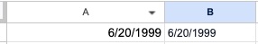
How to tell: Real dates are right-aligned in the cell by default. Text that looks like a date is left-aligned. You can also try =ISNUMBER(A1) — it returns TRUE for real dates and FALSE for text.
Fix 1: DATEVALUE() — For Standard Date Strings
=DATEVALUE("04/13/2026")
This converts text in most common date formats to a proper date. It follows your spreadsheet's locale, so 04/13/2026 is April 13 in US locale but would fail in UK locale (which expects DD/MM/YYYY).
Fix 2: Parse Non-Standard Formats Manually
If your dates are in a format like 13-Apr-2026 or 2026.04.13, you may need to extract the parts:
=DATE(RIGHT(A1,4), MATCH(MID(A1,4,3),{"Jan","Feb","Mar","Apr","May","Jun","Jul","Aug","Sep","Oct","Nov","Dec"},0), LEFT(A1,2))
Or for YYYY.MM.DD:
=DATE(LEFT(A1,4), MID(A1,6,2), RIGHT(A1,2))
Fix 3: Find and Replace Trick
For dates stored as text in the correct format (they just aren't recognized):
- Select the column
- Go to Format → Number → Date (set the format first)
- Open Edit → Find and replace
- Find:
/Replace with:/(same character) - Click Replace all
This forces Google Sheets to re-evaluate each cell, and it will often recognize the values as dates.
How to Change Your Date Locale
Google Sheets uses your spreadsheet's locale to determine the default date format. If dates keep showing in the wrong format (e.g., MM/DD when you want DD/MM), change your locale:
- Go to File → Settings
- Under General, find Locale
- Choose your country (e.g., "United Kingdom" for DD/MM/YYYY or "United States" for MM/DD/YYYY)
- Click Save settings
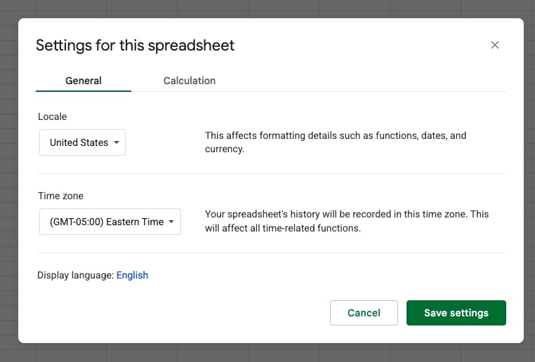
This affects the default format for new dates, number formatting (comma vs period for decimals), and currency symbols.
Common Date Formulas
Beyond formatting, here are the date formulas you'll use most often:
| What you need | Formula | Example result |
|---|---|---|
| Today's date | =TODAY() | 04/13/2026 |
| Current date and time | =NOW() | 04/13/2026 14:30:00 |
| Days between two dates | =DATEDIF(A1,B1,"D") | 30 |
| Months between two dates | =DATEDIF(A1,B1,"M") | 1 |
| Add days to a date | =A1+30 | (30 days later) |
| Add months to a date | =EDATE(A1,3) | (3 months later) |
| First day of the month | =DATE(YEAR(A1),MONTH(A1),1) | 04/01/2026 |
| Last day of the month | =EOMONTH(A1,0) | 04/30/2026 |
| Day of the week (number) | =WEEKDAY(A1) | 2 (Monday) |
| Day of the week (name) | =TEXT(A1,"DDDD") | Monday |
| Quarter | =ROUNDUP(MONTH(A1)/3,0) | 2 |
| Extract year | =YEAR(A1) | 2026 |
| Extract month | =MONTH(A1) | 4 |
| Extract day | =DAY(A1) | 13 |
Fixing Common Date Problems
Dates won't sort correctly
If dates sort as 1, 10, 11... instead of 1, 2, 3..., they're stored as text. See How to Convert Text to Dates above.
Dates show as numbers (like 46117)
Google Sheets stores dates as serial numbers internally. If you see a number instead of a date, select the cell and go to Format → Number → Date. The number 46117 corresponds to April 13, 2026 (days since December 30, 1899).
MM/DD and DD/MM confusion
This happens when your spreadsheet locale doesn't match your date format. 04/05/2026 could be April 5 or May 4 depending on locale. Change your locale under File → Settings, or use the unambiguous ISO format YYYY-MM-DD to avoid confusion entirely.
DATEVALUE() returns an error
DATEVALUE() requires text in a format that matches your spreadsheet locale. If your locale is US and the date text is in DD/MM/YYYY format, it will fail. Either change your locale or parse the date manually with DATE().
Dates from form submissions are wrong
If you're collecting dates via HTML forms and they're appearing incorrectly in Google Sheets, the issue is usually a timezone or format mismatch. When using Sheet Monkey to submit forms to Google Sheets, timestamps are added automatically using date and time fields. Format the timestamp column once, and all future submissions inherit the format.
Date Formats by Region
Different regions use different default date formats. Here's a quick reference:
| Region | Default Format | TEXT() Formula |
|---|---|---|
| United States | MM/DD/YYYY | =TEXT(A1,"MM/DD/YYYY") |
| United Kingdom | DD/MM/YYYY | =TEXT(A1,"DD/MM/YYYY") |
| Germany | DD.MM.YYYY | =TEXT(A1,"DD.MM.YYYY") |
| Japan | YYYY/MM/DD | =TEXT(A1,"YYYY/MM/DD") |
| ISO 8601 (international) | YYYY-MM-DD | =TEXT(A1,"YYYY-MM-DD") |
| China | YYYY年MM月DD日 | =TEXT(A1,"YYYY年MM月DD日") |
When collaborating across regions, use ISO 8601 (YYYY-MM-DD) to avoid ambiguity. It sorts correctly as text, is universally understood, and is the standard for APIs and data interchange.
Using Date Formats with Form Submissions
If you're collecting data through HTML forms into Google Sheets, proper date formatting matters for keeping your data clean.
Sheet Monkey automatically adds submission timestamps when forms are submitted. You can also collect date inputs from form fields — they'll appear in your sheet in whatever format the browser sends them (usually YYYY-MM-DD for <input type="date">).
Tips for clean date data from forms:
- Format your header row first. Sheet Monkey copies formatting from the previous row, so format your timestamp column once and all future submissions inherit it.
- Use
<input type="date">in your HTML. This gives users a date picker and sends dates in ISO format, avoiding locale issues. - Need a quick form? Grab a ready-made form template from our template library or use the drag-and-drop form builder to create one without writing code.
FAQ
How do I change the date format in Google Sheets?
Select your cells, go to Format → Number, and choose a date format. For custom formats, click "Custom number format" and enter a format string like DD/MM/YYYY or YYYY-MM-DD. You can also use the TEXT() function: =TEXT(A1,"MM/DD/YYYY").
How do I convert text to a date in Google Sheets?
Use =DATEVALUE(A1) if the text is in a standard date format matching your locale. For non-standard formats, parse the components manually with =DATE(year, month, day) by extracting each part with LEFT(), MID(), and RIGHT().
Why are my dates showing as numbers? Google Sheets stores dates as serial numbers (days since December 30, 1899). If you see a number like 46117 instead of a date, select the cell and apply a date format: Format → Number → Date.
How do I change the date format from DD/MM/YYYY to MM/DD/YYYY?
Go to File → Settings and change the Locale to "United States" for MM/DD/YYYY or "United Kingdom" for DD/MM/YYYY. This changes the default format for the entire spreadsheet. For individual cells, use a custom number format or the TEXT() function.
Can I use dates in calculations in Google Sheets?
Yes — as long as the dates are actual date values (not text). You can subtract two dates to get the number of days between them (=B1-A1), add days (=A1+30), or use functions like DATEDIF(), EDATE(), and EOMONTH() for more complex calculations.
What is the best date format for Google Sheets?
For data that will be sorted, filtered, or used in formulas, keep dates as actual date values (not text) and format them however you prefer using Format → Number. For international collaboration or data exports, ISO 8601 (YYYY-MM-DD) is the safest choice because it's unambiguous and sorts correctly.
Need to connect HTML forms to Google Sheets? Check out our guide on how to submit HTML forms to Google Sheets, browse our form template library, or try the free form builder for Google Sheets.