How to track your ad campaign conversion with Carrd and Google Sheets

UTM codes, also known as UTM parameters or UTM tags, are snippets of text added to a URL to track and analyze the effectiveness of marketing campaigns and sources. If you’re using a Carrd form with Sheet Monkey to store your conversions in a Google Sheet, the good news is that you can automatically track the campaign performance with just a few extra steps and no additional tools.

1. Turn on UTM tracking in your Carrd form:

When building your Carrd form, check “Collect UTM parameters” and Carrd will automatically forward the campaign parameters to Sheet Monkey and Google Sheets.

Note: You must have Carrd's form method set to "AJAX" not "POST" or "GET" to collect the UTM parameters.

Learn more about Carrd’s support for UTM parameters: Using UTM Parameters - Sites - Documentation - Carrd

Note: If you haven’t already, make sure that your Carrd form is pointed to your Sheet Monkey endpoint. How to submit Carrd forms to Google Sheets

2. Use a the Google Sheets QUERY function to summarize your data

Once you have your Carrd form configured and results are coming in, the data will look something like this:

Now that you’re getting data, you probably want to know exactly which ad is performing the best. The way to do this is with the QUERY function in Google Sheets.

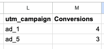
With the data above, this query will yield the following results:

=QUERY(A1:I8, "SELECT F, COUNT(F) WHERE F IS NOT NULL GROUP BY F LABEL COUNT(F) 'Conversions'", 1)

Bingo!

Now if this QUERY expression looks a little confusing, let’s break it down:

• A1:H8 This means select columns A - H and rows 1 through 8. You’ll need to adjust this in your own sheet to select all your columns and rows, depending on how much data you have.
• "SELECT F, COUNT(F) WHERE F IS NOT NULL GROUP BY F LABEL COUNT(F) 'Conversions'" This means select our “utm_campaign” column (F) and how many times it appears in the rows and put that number in a column called “Conversions”.
• 1 This just means to start at the second row. I.E., don’t count the headers row.

You can adjust the column depending on what you wanted to group your results by. For example, say I wanted to see which term was performing the best, I would rewrite the query for column G like this:

”SELECT G, COUNT(G) WHERE F IS NOT NULL GROUP BY G LABEL COUNT(G) 'Conversions'"

and that would yield the following results:

3. Next steps: Add a little visualization

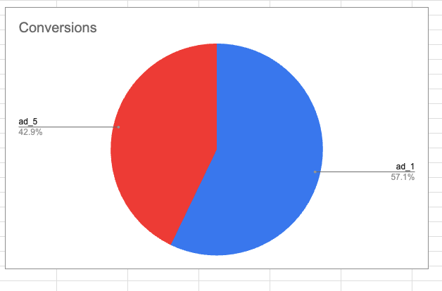
If you want make this even easier, Google Sheets comes with some great charts. Here’s how:

• Select the results that your query generated
• Click Insert → Chart

A chart will immediately be inserted alongside your data.

This is just scratching the surface of what you can do with Google Sheets and building marketing campaigns that convert. Hopefully this has whet your appetite.